statmechcrack.isotensional

A module for the crack model in the isotensional ensemble.

This module consist of the class CrackIsotensional which contains methods for computing quantities in the isotensional (constant force) thermodynamic ensemble.

class CrackIsotensional(**kwargs)

Bases: CrackIsometric

The crack model class for the isotensional ensemble.

Z_0_isotensional(p, lambda_)

The nondimensional isotensional partition function as a function of the nondimensional end force for the reference system,

\[Z_0(p,\boldsymbol{\lambda}) = Z_b(p,\lambda_1,\lambda_2) e^{-\beta U_{01}(\boldsymbol{\lambda})}.\]

Parameters:

• p (array_like) – The nondimensional end force.

• lambda (array_like) – The intact bond stretches.

Returns:

The nondimensional isotensional partition function.

Return type:

numpy.ndarray

Example

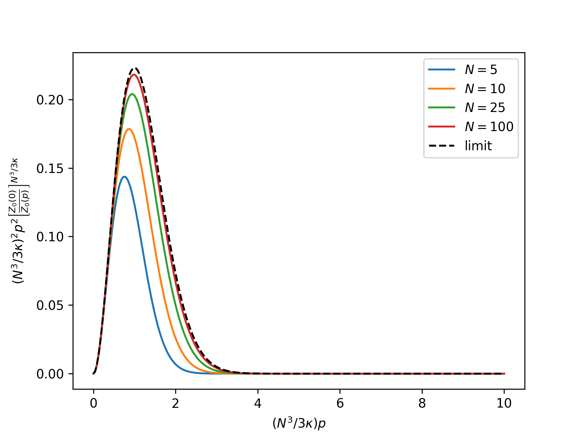
Plot the rescaled nondimensional equilibrium radial distribution as a function of the nondimensional end force for the reference system in the isotensional ensemble for an increasing number of broken bonds \(N\) and compare to the thermodynamic limit:

>>> import numpy as np
>>> import matplotlib.pyplot as plt
>>> from statmechcrack import CrackIsotensional
>>> rp = np.linspace(0, 10, 250)
>>> _ = plt.figure()
>>> for N in [5, 10, 25, 100]:
...     model = CrackIsotensional(N=N)
...     p = 3*model.kappa/N**3*rp
...     r_Z_0 = (model.Z_0_isotensional(0, [1, 1])
...         / model.Z_0_isotensional(p, [1, 1])
...     )**(model.N**3/3/model.kappa)
...     _ = plt.plot(rp, rp**2*r_Z_0, label='$N=$'+str(N))
>>> _ = plt.plot(rp, rp**2*np.exp(-rp*(rp/2 + 1)),
...              'k--', label='limit')
>>> _ = plt.xlabel(r'$(N^3/3\kappa)p$')
>>> _ = plt.ylabel(r'$(N^3/3\kappa)^2p^2$' +
...     r'$\left[\frac{Z_0(0)}{Z_0(p)}\right]^{N^3/3\kappa}$')
>>> _ = plt.legend()
>>> plt.show()

Z_b_isotensional(p, lambda_)

The nondimensional isotensional partition function as a function of the nondimensional end separation for the isolated bending system,

\[Z_b(p,\lambda_1,\lambda_2) = \sqrt{\frac{(2\pi)^{N+1}}{\det\mathbf{H}}} \,e^{\frac{1}{2}\mathbf{g}^T\cdot\mathbf{H}^{-1}\cdot\mathbf{g}-f},\]

where \(\mathbf{H}\), the nondimensional Hessian of the total potential energy for the isolated bending system, and \(\mathbf{g}\) and \(f\) are

\[\mathbf{g}(p,\lambda_1,\lambda_2) = \kappa\left( p/\kappa, 0, \ldots, 0, -\lambda_1, 4\lambda_1 - \lambda_2 \right)^T,\]

\[f(\lambda_1,\lambda_2) = \frac{\kappa}{2}\left[\lambda_1^2 + \left(2\lambda_1 - \lambda_2\right)^2\right] .\]

Parameters:

• p (array_like) – The nondimensional end force.

• lambda (array_like) – The intact bond stretches.

Returns:

The nondimensional isotensional partition function.

Return type:

numpy.ndarray

Z_isotensional(p, transition_state=False)

The nondimensional isotensional partition function as a function of the nondimensional end force,

\[Z(p) = \int d\lambda \ Z_0(p,\boldsymbol{\lambda}) e^{-\beta U_1(\boldsymbol{\lambda})},\]

approximated using the asymptotic relation

\[Z(p) \sim Z_0(p, \hat{\boldsymbol{\lambda}}) \prod_{j=1}^M \sqrt{\frac{2\pi}{\beta u''(\hat{\lambda}_j)}} \, e^{-\beta u(\hat{\lambda}_j)},\]

which is valid for \(\varepsilon\gg 1\), where \(\hat{\boldsymbol{\lambda}}\) is from minimizing \(\beta\Pi\).

Parameters:

• p (array_like) – The nondimensional end force.

• approach (str, optional, default='asymptotic') – The calculation approach.

• transition_state (bool, optional, default=False) – Whether or not to calculate in the transition state.

Example

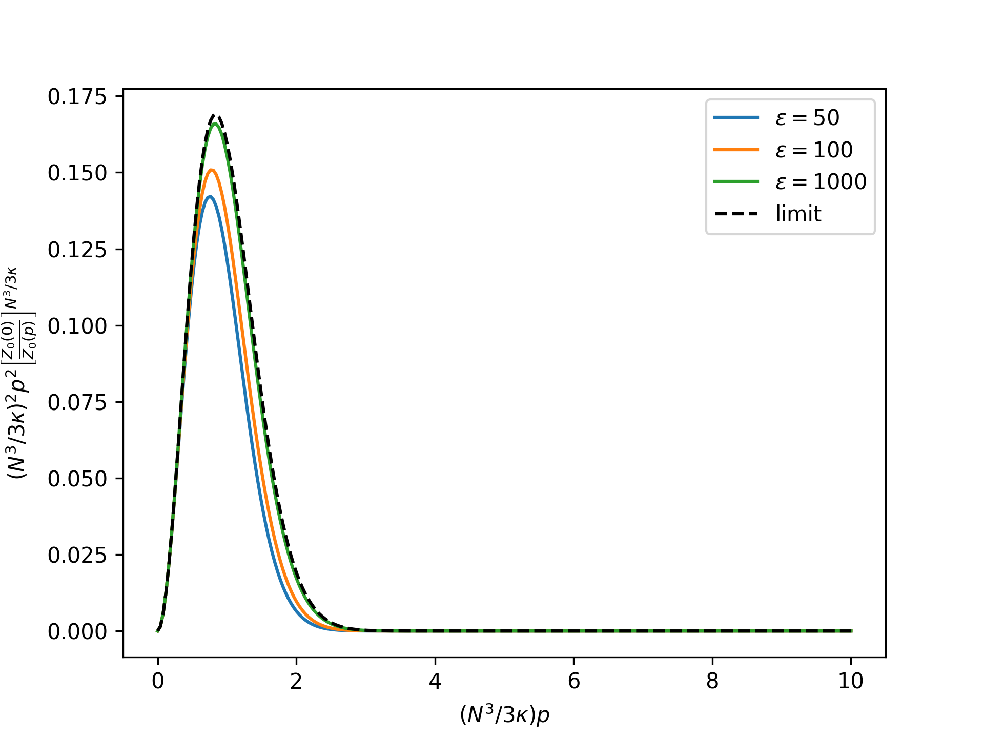
Plot the rescaled nondimensional equilibrium radial distribution as a function of the nondimensional end force in the isotensional ensemble for an increasing nondimensional bond energy and compare to the limit given by the reference system:

>>> import numpy as np
>>> import matplotlib.pyplot as plt
>>> from statmechcrack import CrackIsotensional
>>> rp = np.linspace(0, 10, 250)
>>> _ = plt.figure()
>>> for varepsilon in [50, 100, 1000]:
...     model = CrackIsotensional(varepsilon=varepsilon)
...     p = 3*model.kappa/model.N**3*rp
...     r_Z = (model.Z_isotensional(0)/model.Z_isotensional(p)
...     )**(model.N**3/3/model.kappa)
...     _ = plt.plot(rp, rp**2*r_Z,
...                  label=r'$\varepsilon=$'+str(varepsilon))
>>> r_Z_0 = (model.Z_0_isotensional(0, [1, 1])
...     / model.Z_0_isotensional(p, [1, 1])
... )**(model.N**3/3/model.kappa)
>>> _ = plt.plot(rp, rp**2*r_Z_0, 'k--', label='limit')
>>> _ = plt.xlabel(r'$(N^3/3\kappa)p$')
>>> _ = plt.ylabel(r'$(N^3/3\kappa)^2p^2$' +
...     r'$\left[\frac{Z_0(0)}{Z_0(p)}\right]^{N^3/3\kappa}$')
>>> _ = plt.legend()
>>> plt.show()

Returns:

The nondimensional isotensional partition function.

Return type:

numpy.ndarray

beta_G_0_abs_isotensional(p, lambda_)

The absolute nondimensional Gibbs free energy as a function of the nondimensional end force for the reference system,

\[\beta G_0(p,\boldsymbol{\lambda}) = -\ln Z_0(p,\boldsymbol{\lambda}) = \beta G_b(p,\lambda_1,\lambda_2) + \beta U_{01}(\boldsymbol{\lambda}).\]

Parameters:

• p (array_like) – The nondimensional end force.

• lambda (array_like) – The intact bond stretches.

Returns:

The absolute nondimensional Gibbs free energy.

Return type:

numpy.ndarray

beta_G_0_isotensional(p, lambda_)

The relative nondimensional Gibbs free energy as a function of the nondimensional end force for the reference system,

\[\beta\Delta G_0(p,\boldsymbol{\lambda}) = \beta G_0(p,\boldsymbol{\lambda}) - \beta G_0(0,\boldsymbol{\lambda}).\]

Parameters:

• p (array_like) – The nondimensional end force.

• lambda (array_like) – The intact bond stretches.

Returns:

The relative nondimensional Gibbs free energy.

Return type:

numpy.ndarray

Example

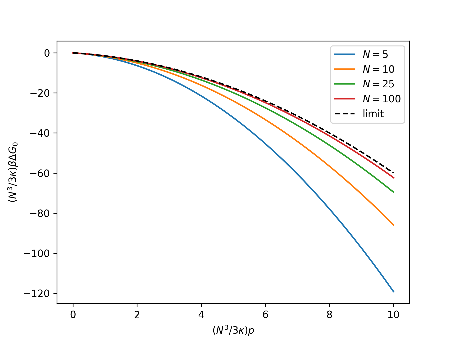
Plot the rescaled nondimensional relative Gibbs free energy as a function of the rescaled nondimensional end force for the reference system in the isotensional ensemble for an increasing number of broken bonds \(N\) and compare to the thermodynamic limit:

>>> import numpy as np
>>> import matplotlib.pyplot as plt
>>> from statmechcrack import CrackIsotensional
>>> rp = np.linspace(0, 10, 33)
>>> _ = plt.figure()
>>> for N in [5, 10, 25, 100]:
...     model = CrackIsotensional(N=N)
...     p = 3*model.kappa/N**3*rp
...     beta_G_0 = \
...         model.beta_G_0_isotensional(p, [1, 1])
...     _ = plt.plot(rp, N**3/3/model.kappa*beta_G_0,
...                  label='$N=$'+str(N))
>>> _ = plt.plot(rp, -rp*(rp/2 + 1), 'k--', label='limit')
>>> _ = plt.xlabel(r'$(N^3/3\kappa)p$')
>>> _ = plt.ylabel(r'$(N^3/3\kappa)\beta\Delta G_0$')
>>> _ = plt.legend()
>>> plt.show()

beta_G_abs_isotensional(p, approach='asymptotic', transition_state=False)

The absolute nondimensional Gibbs free energy as a function of the nondimensional end force,

\[\beta G(p) = -\ln Z(p).\]

Parameters:

• p (array_like) – The nondimensional end force.

• approach (str, optional, default='asymptotic') – The calculation approach.

• transition_state (bool, optional, default=False) – Whether or not to calculate in the transition state.

Returns:

The absolute nondimensional Gibbs free energy.

Return type:

numpy.ndarray

beta_G_b_abs_isotensional(p, lambda_)

The absolute nondimensional Gibbs free energy as a function of the nondimensional end force for the isolated bending system,

\[\beta G_b(p,\lambda_1,\lambda_2) = -\ln Z_b(p,\lambda_1,\lambda_2).\]

Parameters:

• p (array_like) – The nondimensional end force.

• lambda (array_like) – The intact bond stretches.

Returns:

The absolute nondimensional Gibbs free energy.

Return type:

numpy.ndarray

beta_G_b_isotensional(p, lambda_)

The relative nondimensional Gibbs free energy as a function of the nondimensional end force for the isolated bending system,

\[\beta\Delta G_b(p,\lambda_1,\lambda_2) = \beta G_b(p,\lambda_1,\lambda_2) - \beta G_b(0,\lambda_1,\lambda_2).\]

In the thermodynamic limit of a large number of broken bonds \(N\), this function has the asymptotic relation

\[\beta\Delta G_b(p,\lambda_1,\lambda_2) \sim -\frac{N^3}{6\kappa}\,p^2 - p \quad\text{for }N\gg 1.\]

Parameters:

• p (array_like) – The nondimensional end force.

• lambda (array_like) – The intact bond stretches.

Returns:

The relative nondimensional Gibbs free energy.

Return type:

numpy.ndarray

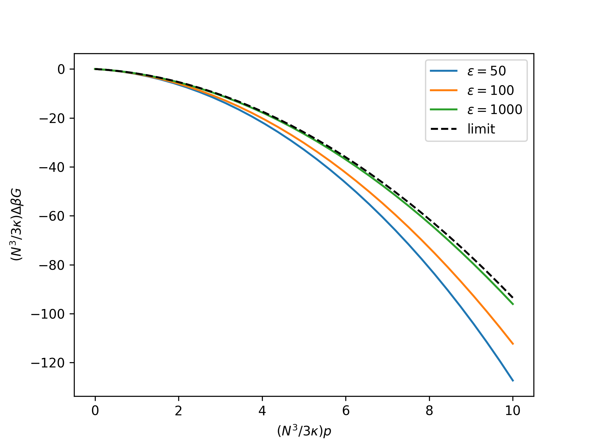
beta_G_isotensional(p, approach='asymptotic', **kwargs)

The relative nondimensional Gibbs free energy as a function of the nondimensional end force,

\[\beta\Delta G(p) = \beta G(p) - \beta G(0).\]

Parameters:

• p (array_like) – The nondimensional end force.

• approach (str, optional, default='asymptotic') – The calculation approach.

• **kwargs – Arbitrary keyword arguments. Passed to beta_G_isotensional_monte_carlo().

Returns:

The relative nondimensional Gibbs free energy.

Return type:

numpy.ndarray

Example

Plot the rescaled nondimensional relative Gibbs free energy as a function of the rescaled nondimensional end force in the isotensional ensemble for an increasing nondimensional bond energy and compare to the limit given by the reference system:

>>> import numpy as np
>>> import matplotlib.pyplot as plt
>>> from statmechcrack import CrackIsotensional
>>> rp = np.linspace(0, 10, 33)
>>> _ = plt.figure()
>>> for varepsilon in [50, 100, 1000]:
...     model = CrackIsotensional(varepsilon=varepsilon)
...     p = 3*model.kappa/model.N**3*rp
...     beta_G = model.beta_G_isotensional(
...         p, approach='asymptotic')
...     _ = plt.plot(rp, model.N**3/3/model.kappa*beta_G,
...                  label=r'$\varepsilon=$'+str(varepsilon))
>>> beta_G_0 = model.beta_G_0_isotensional(p, [1, 1])
>>> _ = plt.plot(rp, model.N**3/3/model.kappa*beta_G_0,
...              'k--', label='limit')
>>> _ = plt.xlabel(r'$(N^3/3\kappa)p$')
>>> _ = plt.ylabel(r'$(N^3/3\kappa)\Delta\beta G$')
>>> _ = plt.legend()
>>> plt.show()

k_0_isotensional(p, lambda_)

The nondimensional forward reaction rate coefficient as a function of the nondimensional end force for the reference system in the isotensional ensemble.

Parameters:

• p (array_like) – The nondimensional end force.

• lambda (array_like) – The intact bond stretches.

Returns:

The nondimensional forward reaction rate.

Return type:

numpy.ndarray

k_b_isotensional(p, lambda_)

The nondimensional forward reaction rate coefficient as a function of the nondimensional end force for the isolated bending system in the isotensional ensemble.

Parameters:

• p (array_like) – The nondimensional end force.

• lambda (array_like) – The intact bond stretches.

Returns:

The nondimensional forward reaction rate.

Return type:

numpy.ndarray

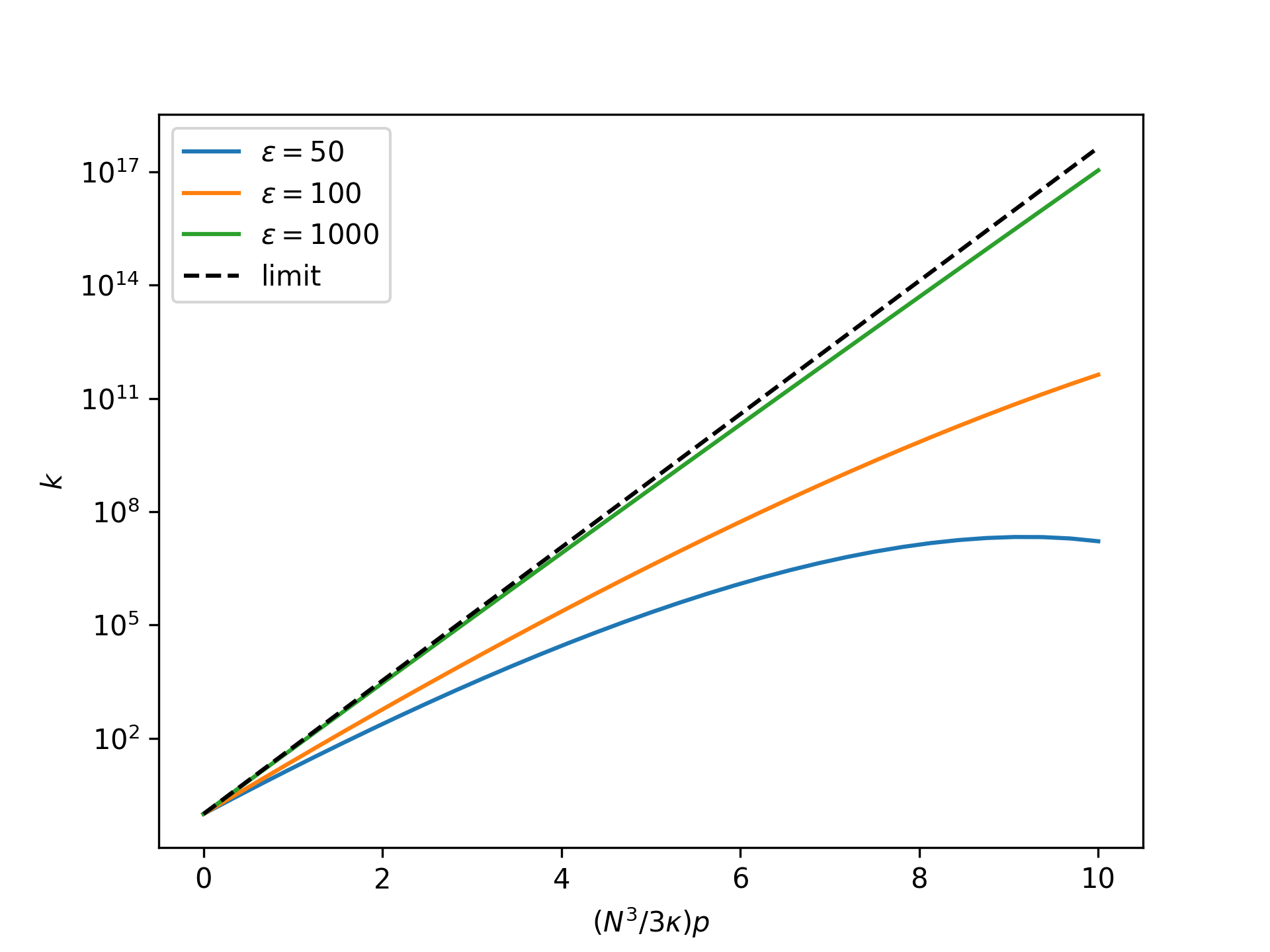
k_isotensional(p, approach='asymptotic', **kwargs)

The nondimensional forward reaction rate coefficient as a function of the nondimensional end force in the isotensional ensemble.

Parameters:

• p (array_like) – The nondimensional end force.

• approach (str, optional, default='asymptotic') – The calculation approach.

Returns:

The nondimensional forward reaction rate.

Return type:

numpy.ndarray

Example

Plot the nondimensional forward reaction rate coefficient as a function of the nondimensional end force in the isotensional ensemble for an increasing nondimensional bond energy and compare to the limit given by the reference system:

>>> import numpy as np
>>> import matplotlib.pyplot as plt
>>> from statmechcrack import CrackIsotensional
>>> rp = np.linspace(0, 10, 33)
>>> _ = plt.figure()
>>> for varepsilon in [50, 100, 1000]:
...     model = CrackIsotensional(varepsilon=varepsilon)
...     p = 3*model.kappa/model.N**3*rp
...     _ = plt.semilogy(
...         rp, model.k_isotensional(p),
...         label=r'$\varepsilon=$'+str(varepsilon))
>>> _ = plt.semilogy(rp, model.k_0_isotensional(p, [1, 1]),
...                  'k--', label='limit')
>>> _ = plt.xlabel(r'$(N^3/3\kappa)p$')
>>> _ = plt.ylabel(r'$k$')
>>> _ = plt.legend()
>>> plt.show()

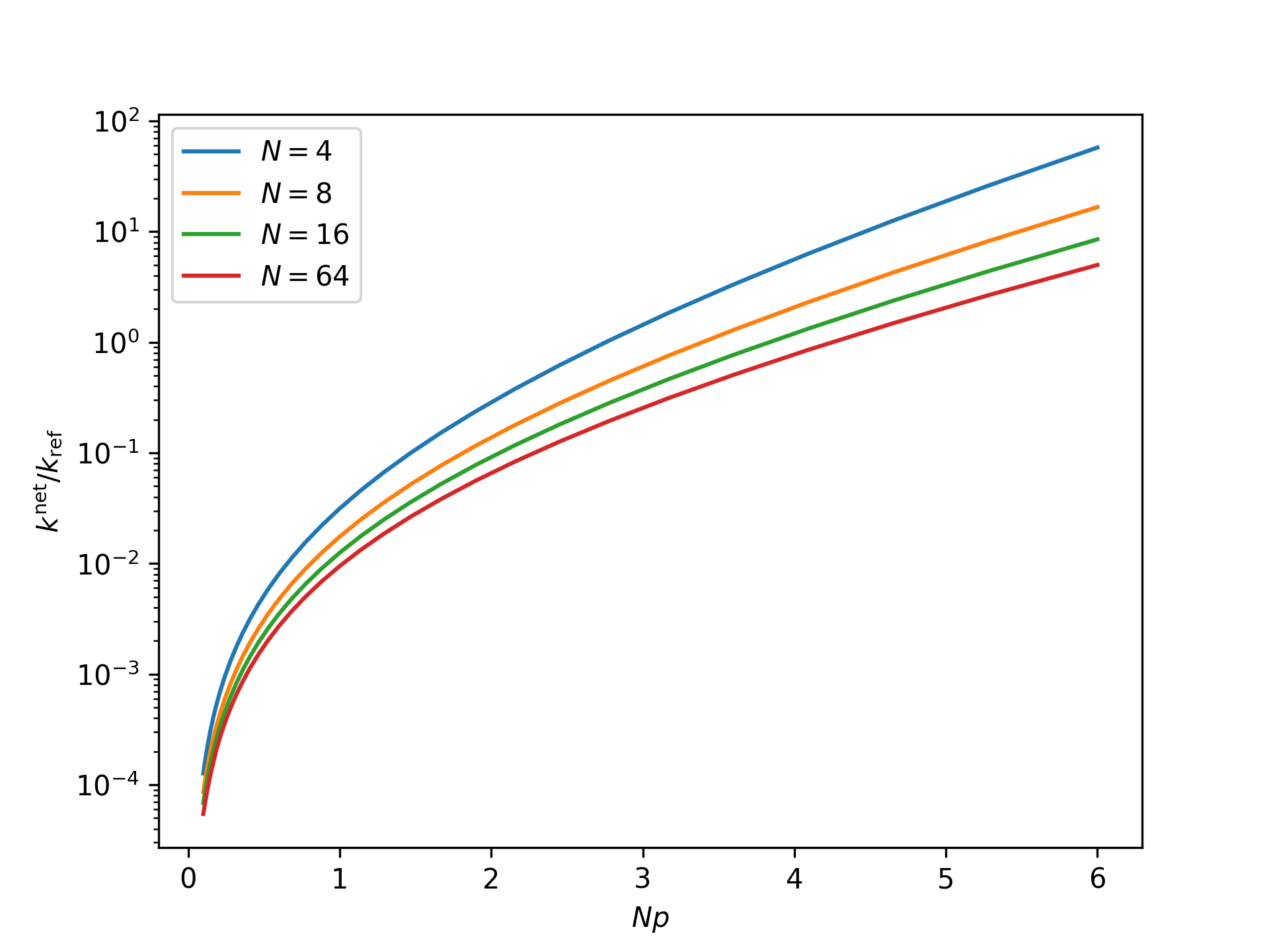
k_net_isotensional(p)

The nondimensional net reaction rate coefficient as a function of the nondimensional end force in the isotensional ensemble.

Parameters:

p (array_like) – The nondimensional end force.

Returns:

The nondimensional net reaction rate.

Return type:

numpy.ndarray

Example

Plot the nondimensional net reaction rate coefficient as a function of the nondimensional end force in the isotensional ensemble for an increasing system size:

>>> import numpy as np
>>> import matplotlib.pyplot as plt
>>> from statmechcrack import Crack
>>> Np = np.logspace(-1, np.log(6)/np.log(10), 33)
>>> _ = plt.figure()
>>> for N in [4, 8, 16, 64]:
...     model = Crack(N=N)
...     _ = plt.semilogy(
...         Np, model.k_net(Np/N, ensemble='isotensional'),
...         label=r'$N=$'+str(N))
>>> _ = plt.xlabel(r'$Np$')
>>> _ = plt.ylabel(r'$k^\mathrm{net}/k_\mathrm{ref}$')
>>> _ = plt.legend()
>>> plt.show()

k_rev_isotensional(p)

The nondimensional reverse reaction rate coefficient as a function of the nondimensional end force in the isotensional ensemble.

Parameters:

p (array_like) – The nondimensional end force.

Returns:

The nondimensional reverse reaction rate.

Return type:

numpy.ndarray

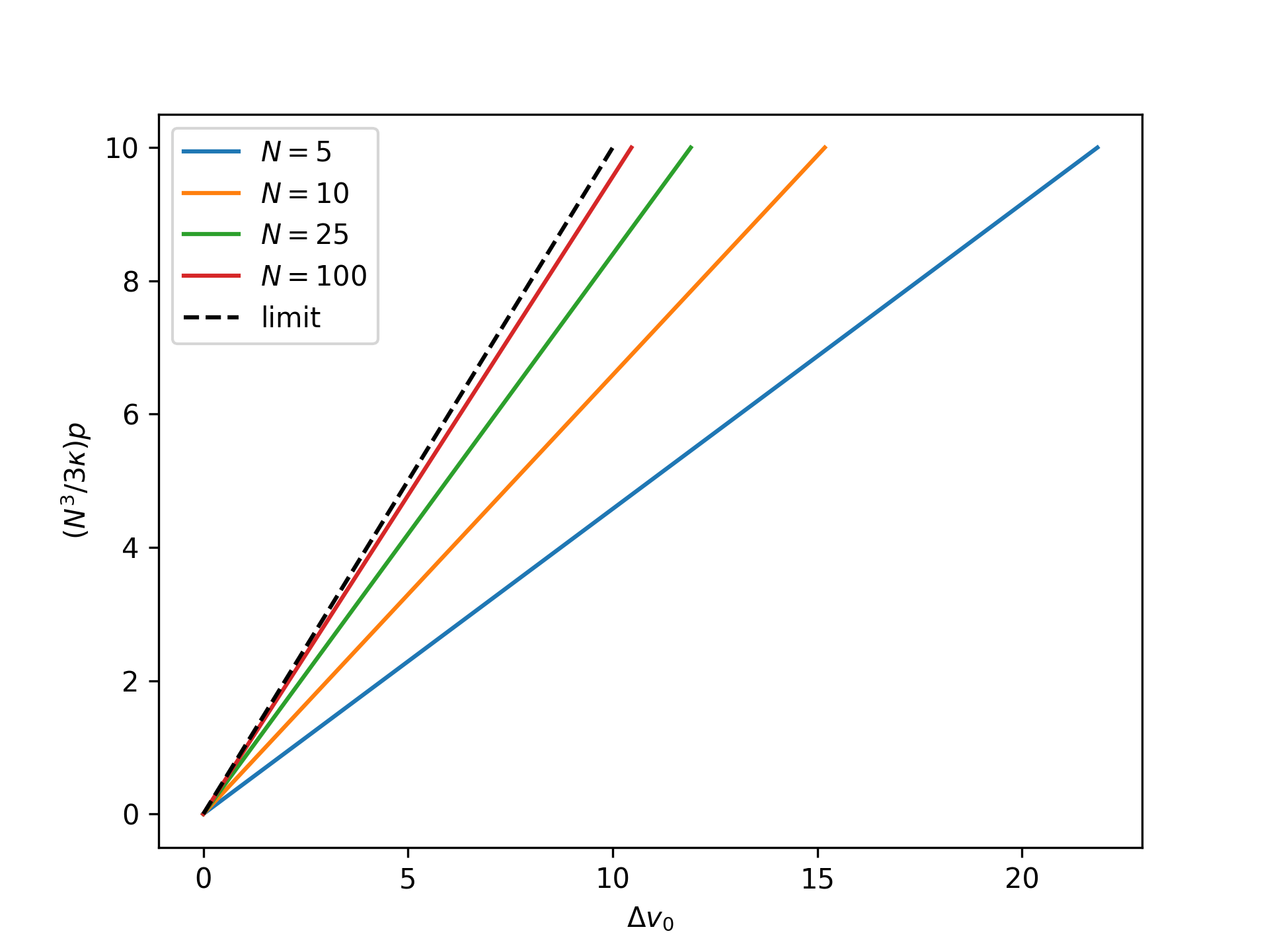
v_0_isotensional(p, lambda_)

The nondimensional end separation as a function of the nondimensional end force for the reference system in the isotensional ensemble,

\[v_0(p,\lambda_1,\lambda_2) = -\frac{\partial}{\partial p} \,\beta G_0(p,\lambda_1,\lambda_2) = v_b(p,\lambda_1,\lambda_2).\]

Parameters:

• p (array_like) – The nondimensional end force.

• lambda (list) – The stretch of the first two intact bonds.

Returns:

The nondimensional end separation.

Return type:

numpy.ndarray

Example

Plot the nondimensional end separation as a function of the rescaled nondimensional end force for the reference system in the isotensional ensemble for an increasing number of broken bonds \(N\) and compare to the thermodynamic limit:

>>> import numpy as np
>>> import matplotlib.pyplot as plt
>>> from statmechcrack import CrackIsotensional
>>> rp = np.linspace(0, 10, 33)
>>> _ = plt.figure()
>>> for N in [5, 10, 25, 100]:
...     model = CrackIsotensional(N=N)
...     p = 3*model.kappa/N**3*rp
...     v_0 = model.v_0_isotensional(p, [1, 1])
...     _ = plt.plot(v_0 - 1, rp, label='$N=$'+str(N))
>>> _ = plt.plot(rp, rp, 'k--', label='limit')
>>> _ = plt.xlabel(r'$\Delta v_0$')
>>> _ = plt.ylabel(r'$(N^3/3\kappa)p$')
>>> _ = plt.legend()
>>> plt.show()

v_b_isotensional(p, lambda_)

The nondimensional end separation as a function of the nondimensional end force for the isolated bending system in the isotensional ensemble,

\[v_b(p,\lambda_1,\lambda_2) = -\frac{\partial}{\partial p} \,\beta G_b(p,\lambda_1,\lambda_2).\]

In the thermodynamic limit of a large number of broken bonds \(N\), this function has the asymptotic relation

\[v_b(p,\lambda_1,\lambda_2) \sim v_0 + \frac{N^3}{3\kappa}\,p \quad\text{for }N\gg 1.\]

Parameters:

• p (array_like) – The nondimensional end force.

• lambda (list) – The stretch of the first two intact bonds.

Returns:

The nondimensional end separation.

Return type:

numpy.ndarray

v_isotensional(p, approach='asymptotic', **kwargs)

The nondimensional end separation as a function of the nondimensional end force in the isotensional ensemble,

\[v(p) = -\frac{\partial}{\partial p}\,\beta G(p).\]

Parameters:

• p (array_like) – The nondimensional end force.

• approach (str, optional, default='asymptotic') – The calculation approach.

• **kwargs – Arbitrary keyword arguments. Passed to v_isotensional_monte_carlo().

Returns:

The nondimensional end separation.

Return type:

numpy.ndarray

Example

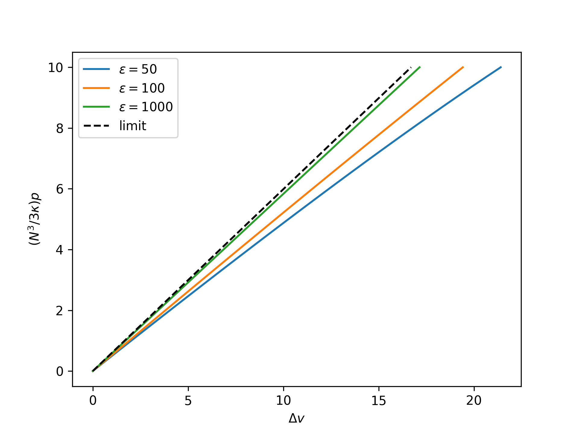
Plot the nondimensional end separation as a function of the rescaled nondimensional end force in the isotensional ensemble for an increasing nondimensional bond energy and compare to the limit given by the reference system:

>>> import numpy as np
>>> import matplotlib.pyplot as plt
>>> from statmechcrack import CrackIsotensional
>>> rp = np.linspace(0, 10, 33)
>>> _ = plt.figure()
>>> for varepsilon in [50, 100, 1000]:
...     model = CrackIsotensional(varepsilon=varepsilon)
...     p = 3*model.kappa/model.N**3*rp
...     v = model.v_isotensional(p, approach='asymptotic')
...     _ = plt.plot(v - 1, rp,
...                  label=r'$\varepsilon=$'+str(varepsilon))
>>> v_0 = model.v_0_isotensional(p, [1, 1])
>>> _ = plt.plot(v_0 - 1, rp, 'k--', label='limit')
>>> _ = plt.xlabel(r'$\Delta v$')
>>> _ = plt.ylabel(r'$(N^3/3\kappa)p$')
>>> _ = plt.legend()
>>> plt.show()