Tutorial

This is a tutorial demonstrating the basics of the Python package statmechcrack.

Model Creation

The crack model is imported from the package as the Crack class,

from statmechcrack import Crack

Instantiating the class creates a particular model instance,

model = Crack()

Keyword arguments allow model features to be selected during instantiation, such as choosing 8 repeat units behind the crack tip and a nondimensional energy scale of 88 ahead of the crack tip:

model = Crack(N=8, varepsilon=88)

Model Methods

A crack model instance has many methods available, such as v, the nondimensional end separation as a function of the nondimensional end force

model.v

<bound method Crack.v of <statmechcrack.core.Crack object at 0x7fb5945fc190>>

model.v(1)

array([4.28297647])

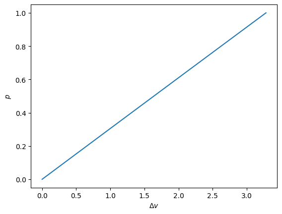
An array of nondimensional forces can be input, and the results plotted:

import numpy as np
import matplotlib.pyplot as plt
from statmechcrack import Crack
model = Crack(N=8, varepsilon=88)
p = np.linspace(0, 1, 100)
plt.plot(model.v(p) - 1, p)
plt.xlabel(r'$\Delta v$')
plt.ylabel(r'$p$')
plt.show()

Thermodynamic Ensembles

Generally, results will differ when either a constant end force or a constant end separation is applied to the crack model system. These are the isotensional and isometric thermodynamic ensembles, respectively. The ensemble can be specified when computing a result using a class method. For example, the nondimensional end force under a nondimensional end separation of 3 (isometric) is not exactly the same force that will cause a nondimensional end separation of 3 in the isotensional ensemble:”

model.p(3, ensemble='isometric')

array([0.60998242])

model.v(0.60998242, ensemble='isotensional')

array([3.00010209])

Thermodynamic Limit

As the model system becomes large (many repeat units), the results from any ensemble tend to converge. This is referred to as the thermodynamic limit.

model = Crack(N=25, M=25, varepsilon=88)
model.p(3, ensemble='isometric')

array([0.03067685])

model.v(0.03067685, ensemble='isotensional')

array([2.99999971])

Calculations Approaches

The coupling between degrees of freedom in this model system prevents thermodynamic functions (the class methods) from being evaluated analytically. Two calculation approaches are provided: an analytic, asymptotically-valid approximation approach, and a Monte Carlo approach. The asymptotic approach is the default. As the bonds ahead of the crack tip become stiff, the asymptotic approach becomes valid:

v = np.linspace(1, 11, 33)
_ = plt.figure()
for varepsilon in [10, 25, 100, 800]:
    model = Crack(varepsilon=varepsilon)
    p = model.p(v, approach='asymptotic')
    _ = plt.plot(v - 1, p, label=r'$\varepsilon=$'+str(varepsilon))
p_0 = model.p_0_isometric(v, [1, 1])
_ = plt.plot(v - 1, p_0, 'k--', label='limit')
_ = plt.xlabel(r'$\Delta v$')
_ = plt.ylabel(r'$p$')
_ = plt.legend()
plt.show()

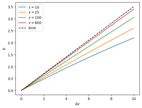
The infinitely-stiff limit is given by the reference system, which is where the bonds ahead of the crack tip are rigidly constrained, and which is analytically solvable in this case.